深度学习之RNN模型

[TOC]

一、简介

序列数据是生活中很常见的一种数据，如一句话、一段时间某个广告位的流量、一连串运动视频的截图等。在这些数据中也有着很多数据挖掘的需求。如下图所示，来自吴恩达Sequence Models的案例。

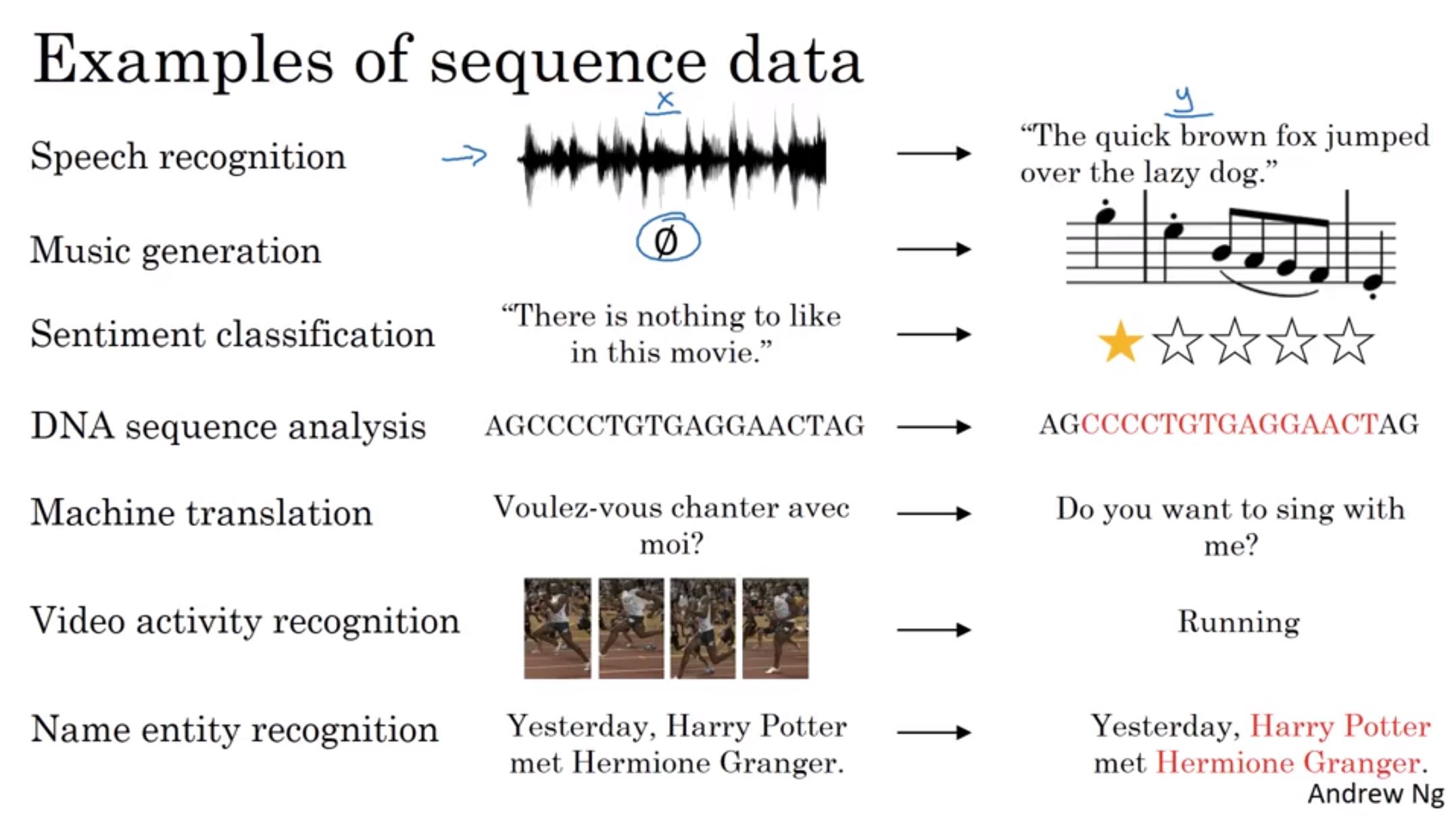
以最后一个命名实体识别为例，我们需要识别文本中的姓名。那么给出一些标注过姓名的数据，如何训练模型来预测未标注的文本中的姓名？这就是序列数据的数据挖掘任务。RNN就是解决这类问题的一种深度学习方法。其全称是Recurrent Neural Networks，中文是递归神经网络。主要解决序列数据的数据挖掘问题。

本文是来自吴恩达《Sequence Models》课程的笔记。

二、为什么需要RNN

首先，我们看一下传统的DNN模型如何解决上述问题。一般来说，我们可以使用如下结构的深度学习网络来为上述问题建模。

首先，我们看一下标注的数据，以上述文本为例，训练集的一句话如下：

Yesterday, Harry Potter met Hermione Granger.

假设每个单词用onhe-hot编码或者词嵌套编码，用x表示，去除标点符号之后，我们可以将上述训练数据表示如下：

数据实例	Yesterday	Harry	Potter	met	Hermione	Granger
输入x	x1	x2	x3	x4	x5	x6
标签y	0	1	1	0	1	1

下面的标签中，值为1的表示该单词是人名，如果是0，则表示非人名。上述数据就是我们的训练数据。对这个数据我们可以构造如下图所示的神经网络：

这里的T_x表示输入数据的个数，T_y表示输出标签的个数。上标表示第几个数据。尽管这个模型也可以为上述案例建模，但是它有两个巨大的问题：

1、在某些任务中，不同的数据中，输入和输出的长度并不是恒定不变的。例如，对于翻译任务来说，原语言的句子和目标语言的句子的长度是不同的，不同的训练数据之间也是不同的。这样的情况，上述模型是不能运行的。
2、其次，在文本中不同位置学习到的特征之间是互相不影响的，这可能会丢失某些重要的数据，因为序列数据中“位置”或者“顺序”信息也很重要。

基于上述两个问题，研究者提出使用RNN模型来解决序列数据的数据挖掘问题。

三、RNN模型框架

RNN的模型结果如下：

从上图可以看到，原来输入数据到标签是从左到右的顺序，现在变成了单个数据点对应输出的结构，且是自下而上的。这里的一层只有一个数据中的一个标签对应关系。例如第一层中是x^{< 1 >}对应了它的输出\hat{y}^{< 1>}。同时，为了给序列之间的数据关系建模，层与层之间用一个变量a连接，这样序列数据中的后一个数据的输入就会把前面的信息给编码进去，进而解决原来模型上不同位置之间特征不共享的问题。

3.1、RNN的前向传播

下面以第一层为例，我们给出RNN的前向传播的公式。每一层的输入和输出都有两个变量。

输入：一个是当前位置的数据x^{< t>}，一个是前一个位置的激活函数输出a^{< t-1>}
输出：一个是预测的标签\hat{y}^{< t>}，一个是本层的激活函数的输出a^{< t>}。

以第一层为例，这里的a^{< 0>}是第一层的输入，一般设置为0即可。首先，我们要计算第一层的权重a^{< 1>}：

a^{< 1>} = g(W_{aa}a^{<0>} + W_{ax}x^{<1>} + b_a)

这里W_{aa}是激活函数相关的权重矩阵，W_{ax}是数据相关的权重矩阵，b_a是偏差。这里的激活函数g通常使用tanh或者是relu。

然后，我们还需要计算第一层的预测的标签：

\hat{y}^{<1>} = g(W_{ya}a^{<1>} + b_y)

这里的W_{ya}是预测相关的权重矩阵，b_y是偏差。这里的激活函数g通常使用sigmoid。

每一层都是如上例所示建模即可得到所有的RNN前向传播的建模结果。当然，我们也可以把计算a的权重矩阵合并，简化成如下形式，即第t层网络的前向传播公式如下：

a^{< t>} = g(W_a [a^{< t-1>}|x^{< t>}] + b_a)

\hat{y}^{< t>} = g(W_y a^{< t>} + b_y)

3.2、RNN的损失函数

一般来说，对于RNN的第t层我们可以定义如下损失函数：

\mathcal{L}^{< t>}(\hat{y}^{< t>},y^{< t>}) = -y^{< t>}\log \hat{y}^{< t>} - (1-y^{< t>})\log (1-\hat{y}^{< t>})

总的最终的损失函数为：

\mathcal{L}(\hat{y},y) = \sum_{t=1}^{T_y}\mathcal{L}^{< t>}(\hat{y}^{< t>},y^{< t>})

3.3、RNN的反向传播

在上面的前向传播中，我们知道每一层有如下变量：W_{aa}、W_{ax}、b_{a}、b_{y}。其主要的计算如下图所示：

四、其他形式的RNN模型

除了上述模型外，我们还有如下图所示的其他形式的RNN结构。

五、核心代码示例

首先，我们写出如下前向传播中一层的计算方法rnn_cell_forward(xt, a_prev, parameters)，其输入是上一层的权重a_prev和这一层的数据xt：

def rnn_cell_forward(xt, a_prev, parameters):
    """
    Implements a single forward step of the RNN-cell as described in Figure (2)

    Arguments:
    xt -- your input data at timestep "t", numpy array of shape (n_x, m).
    a_prev -- Hidden state at timestep "t-1", numpy array of shape (n_a, m)
    parameters -- python dictionary containing:
                        Wax -- Weight matrix multiplying the input, numpy array of shape (n_a, n_x)
                        Waa -- Weight matrix multiplying the hidden state, numpy array of shape (n_a, n_a)
                        Wya -- Weight matrix relating the hidden-state to the output, numpy array of shape (n_y, n_a)
                        ba --  Bias, numpy array of shape (n_a, 1)
                        by -- Bias relating the hidden-state to the output, numpy array of shape (n_y, 1)
    Returns:
    a_next -- next hidden state, of shape (n_a, m)
    yt_pred -- prediction at timestep "t", numpy array of shape (n_y, m)
    cache -- tuple of values needed for the backward pass, contains (a_next, a_prev, xt, parameters)
    """

    # Retrieve parameters from "parameters"
    Wax = parameters["Wax"]
    Waa = parameters["Waa"]
    Wya = parameters["Wya"]
    ba = parameters["ba"]
    by = parameters["by"]

    # compute next activation state using the formula given above
    a_next = np.tanh(np.dot(Waa,a_prev) + np.dot(Wax,xt) + ba)
    # compute output of the current cell using the formula given above
    yt_pred = softmax(np.dot(Wya,a_next) + by)   

    # store values you need for backward propagation in cache
    cache = (a_next, a_prev, xt, parameters)

    return a_next, yt_pred, cache

那么，对于所有的数据，我们需要循环计算上述方法：

def rnn_forward(x, a0, parameters):
    """
    Implement the forward propagation of the recurrent neural network described in Figure (3).

    Arguments:
    x -- Input data for every time-step, of shape (n_x, m, T_x).
    a0 -- Initial hidden state, of shape (n_a, m)
    parameters -- python dictionary containing:
                        Waa -- Weight matrix multiplying the hidden state, numpy array of shape (n_a, n_a)
                        Wax -- Weight matrix multiplying the input, numpy array of shape (n_a, n_x)
                        Wya -- Weight matrix relating the hidden-state to the output, numpy array of shape (n_y, n_a)
                        ba --  Bias numpy array of shape (n_a, 1)
                        by -- Bias relating the hidden-state to the output, numpy array of shape (n_y, 1)

    Returns:
    a -- Hidden states for every time-step, numpy array of shape (n_a, m, T_x)
    y_pred -- Predictions for every time-step, numpy array of shape (n_y, m, T_x)
    caches -- tuple of values needed for the backward pass, contains (list of caches, x)
    """

    # Initialize "caches" which will contain the list of all caches
    caches = []

    # Retrieve dimensions from shapes of x and parameters["Wya"]
    n_x, m, T_x = x.shape
    n_y, n_a = parameters["Wya"].shape


    # initialize "a" and "y" with zeros (≈2 lines)
    a = np.zeros([n_a, m, T_x])
    y_pred = np.zeros([n_y, m, T_x])

    # Initialize a_next (≈1 line)
    a_next = a0

    # loop over all time-steps
    for t in range(T_x):
        # Update next hidden state, compute the prediction, get the cache (≈1 line)
        a_next, yt_pred, cache = rnn_cell_forward(x[:,:,t], a_next, parameters)
        # Save the value of the new "next" hidden state in a (≈1 line)
        a[:,:,t] = a_next
        # Save the value of the prediction in y (≈1 line)
        y_pred[:,:,t] = yt_pred
        # Append "cache" to "caches" (≈1 line)
        caches.append(cache)

    # store values needed for backward propagation in cache
    caches = (caches, x)

    return a, y_pred, caches

后向传播的代码如下：

def rnn_cell_backward(da_next, cache):
    """
    Implements the backward pass for the RNN-cell (single time-step).
    Arguments:
    da_next -- Gradient of loss with respect to next hidden state
    cache -- python dictionary containing useful values (output of rnn_cell_forward())
    Returns:
    gradients -- python dictionary containing:
                        dx -- Gradients of input data, of shape (n_x, m)
                        da_prev -- Gradients of previous hidden state, of shape (n_a, m)
                        dWax -- Gradients of input-to-hidden weights, of shape (n_a, n_x)
                        dWaa -- Gradients of hidden-to-hidden weights, of shape (n_a, n_a)
                        dba -- Gradients of bias vector, of shape (n_a, 1)
    """

    # Retrieve values from cache
    (a_next, a_prev, xt, parameters) = cache

    # Retrieve values from parameters
    Wax = parameters["Wax"]
    Waa = parameters["Waa"]
    Wya = parameters["Wya"]
    ba = parameters["ba"]
    by = parameters["by"]

    ### START CODE HERE ###
    # compute the gradient of tanh with respect to a_next (≈1 line)
    dtanh = (1-a_next*a_next)*da_next

    # compute the gradient of the loss with respect to Wax (≈2 lines)
    dxt = np.dot(Wax.T,  dtanh)
    dWax = np.dot(dtanh,xt.T)

    # compute the gradient with respect to Waa (≈2 lines)
    da_prev = np.dot(Waa.T, dtanh)  
    dWaa = np.dot( dtanh,a_prev.T)

    # compute the gradient with respect to b (≈1 line)
    dba = np.sum( dtanh,keepdims=True,axis=-1)

    ### END CODE HERE ###

    # Store the gradients in a python dictionary
    gradients = {"dxt": dxt, "da_prev": da_prev, "dWax": dWax, "dWaa": dWaa, "dba": dba}

    return gradients

def rnn_backward(da, caches):
    """
    Implement the backward pass for a RNN over an entire sequence of input data.
    Arguments:
    da -- Upstream gradients of all hidden states, of shape (n_a, m, T_x)
    caches -- tuple containing information from the forward pass (rnn_forward)

    Returns:
    gradients -- python dictionary containing:
                        dx -- Gradient w.r.t. the input data, numpy-array of shape (n_x, m, T_x)
                        da0 -- Gradient w.r.t the initial hidden state, numpy-array of shape (n_a, m)
                        dWax -- Gradient w.r.t the input's weight matrix, numpy-array of shape (n_a, n_x)
                        dWaa -- Gradient w.r.t the hidden state's weight matrix, numpy-arrayof shape (n_a, n_a)
                        dba -- Gradient w.r.t the bias, of shape (n_a, 1)
    """

    ### START CODE HERE ###

    # Retrieve values from the first cache (t=1) of caches (≈2 lines)
    (caches, x) = caches
    (a1, a0, x1, parameters) = caches[0]

    # Retrieve dimensions from da's and x1's shapes (≈2 lines)
    n_a, m, T_x = da.shape
    n_x, m = x1.shape 

    # initialize the gradients with the right sizes (≈6 lines)
    dx = np.zeros((n_x, m, T_x)) 
    dWax = np.zeros((n_a, n_x))
    dWaa = np.zeros((n_a, n_a))
    dba = np.zeros((n_a, 1)) 
    da0 = np.zeros((n_a, m))
    da_prevt = np.zeros((n_a, m))  

    # Loop through all the time steps
    for t in reversed(range(T_x)):
        # Compute gradients at time step t. Choose wisely the "da_next" and the "cache" to use in the backward propagation step. (≈1 line)
        gradients = rnn_cell_backward(da[:, :, t] + da_prevt, caches[t])
        # Retrieve derivatives from gradients (≈ 1 line)
        dxt, da_prevt, dWaxt, dWaat, dbat = gradients["dxt"], gradients["da_prev"], gradients["dWax"], gradients["dWaa"], gradients["dba"]
        # Increment global derivatives w.r.t parameters by adding their derivative at time-step t (≈4 lines)
        dx[:, :, t] = dxt  
        dWax += dWaxt  
        dWaa += dWaat  
        dba += dbat  

    # Set da0 to the gradient of a which has been backpropagated through all time-steps (≈1 line) 
    da0 = None
    ### END CODE HERE ###

    # Store the gradients in a python dictionary
    gradients = {"dx": dx, "da0": da0, "dWax": dWax, "dWaa": dWaa,"dba": dba}

    return gradients